Word Origin Relationship Graph

This post covers an analysis of word origins from a dataset found here. I found the dataset a while back, and it seemed like a good chance to use it to experiment with directed graphs a bit, as the word origins could be reasonably represented in that way.

The Dataset

The dataset was published in 2013, and consists of information mined from Wiktionary, an online dictionary with various information on words from many languages, including definitions, pronunciation, and etymology. The dataset’s homepage links to a short paper going into the methods of data mining in more detail, though the broad view seems to be that it was mostly powered by recursive regular expressions applied to the pages' XML.

The data file itself is tab-delimited, consisting of three columns: the first word, the relationship between the words, and the second word. The dataset contains just over six million entries.

> import pandas as pd
> df = pd.read_csv("etymwn.tsv", sep="\t", header=None, names=["Word1", "Relationship", "Word2"])
> df.head()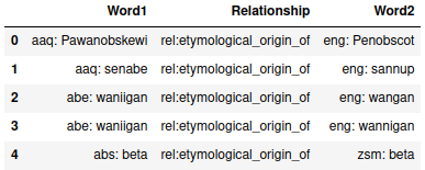

> df.shape
(6031431, 3)

From the view of the head of the dataset, we can see that the text in the word columns also contain the language of the word. As far as I can tell, these are all ISO 639-3 language codes, an international standard of three-letter codes, which will be relied on later when actually viewing the data as a graph.

Exploratory Analysis

First, a little exploration of the data and answering a few questions.

First question: Is the data totally symmetric? That is, for each entry along the lines of “x etymological_origin_of y”, is there a corresponding “y is_derived_from x”?

> df["Word1"].unique().shape
(2886098,)
> df["Word2"].unique().shape
(2880769,)

Different numbers of unique words means that the two columns cannot have the same set of unique words in them, which is a necessary prerequisite for the data being symmetric. As such, it is clearly not symmetric, which is slightly unfortunate since it could make filtering duplicates much easier.

Second question: How many languages are there, and are they the same between the two columns?

> w1_langs = df["Word1"].str.slice(0,3).unique()
> w2_langs = df["Word2"].str.slice(0,3).unique()
> w1_langs.shape
(396,)
> w2_langs.shape
(396,)
> set(w1_langs) == set(w2_langs)
True

A total of 396 languages are present, and the languages are the same between the two word columns. The number of languages means that attempting to show every language in the data on a reasonably-sized graph is probably infeasible.

Third, what do the relationships in the data mean? This one requires a bit more inference, so let’s look at what values exist first:

> df["Relationship"].value_counts()
rel:is_derived_from           2264744
rel:has_derived_form          2264744
rel:etymologically_related     538558
rel:etymological_origin_of     473433
rel:etymology                  473433
rel:variant:orthography         16516
rel:derived                         2
rel:etymologically                  1
Name: Relationship, dtype: int64

To me, only three of the relationships – is_derived_from, has_derived_form, ad etymological_origin_of – seem fairly unambiguous in the direction of the relationship, which is what we’re interested in. Thankfully, the former two of those are the most common entries, and the three unambiguous cases overall count for about 83% of the data, so we shouldn’t have to lose too much data no matter what.

For the remainder, I’m willing to discard the derived and etymologically relationships as they have so few entries. And a quick group-and-count check confirms that there are some word pairs which seem to have multiple relationships listed:

> groupings = df.groupby(["Word1", "Word2"]).size()
> groupings.value_counts()
1    5729121
2     144672
3       4284
4         26
5          2
dtype: int64

Most only appear once, but there are around 150,000 terms which appear more than once, and this doesn’t count rows which have the same meaning but reversed word order (e.g., “A is the origin of B” versus “B is descended from A”). Since some records share words, my hope is that those instances provide enough information that we can impute the ambiguous relationships into unambiguous ones. The below function does the analysis part of that.

> def other_relationship_count(df, relationship):
>     # Look for instances where the word pairs that have the specified
>     # relationship appear in other rows, and return the counts of the
>     # relationships in those other rows
>     subset = df.loc[df["Relationship"] == relationship]
>     relationship_names = subset["Word1"] + subset["Word2"]
>     is_relevant_row = (df["Word1"] + df["Word2"]).isin(relationship_names) & (df["Relationship"] != relationship)
>     return df.loc[is_relevant_row]["Relationship"].value_counts()
> 
> other_relationship_count(df, "rel:etymologically_related")
rel:is_derived_from           17019
rel:has_derived_form          17019
rel:etymology                 13615
rel:etymological_origin_of    13615
rel:variant:orthography          20
Name: Relationship, dtype: int64
> 
> other_relationship_count(df, "rel:etymology")
rel:is_derived_from           46081
rel:etymologically_related    13615
rel:has_derived_form            458
rel:etymological_origin_of      284
rel:variant:orthography           3
rel:derived                       1
Name: Relationship, dtype: int64
> 
> other_relationship_count(df, "rel:variant:orthography")
rel:etymologically_related    20
rel:is_derived_from            8
rel:etymological_origin_of     6
rel:has_derived_form           3
rel:etymology                  3
Name: Relationship, dtype: int64

So etymologically_related is deadlocked between its two highest results, and variant:orthography doesn’t have much to go on, but etymology usually seems to follow one form, at least, so I’m willing to try that replacement.

> df.loc[df["Relationship"] == "rel:etymology", "Relationship"] = "rel:is_derived_from"
> good_relationships = ["rel:is_derived_from", "rel:has_derived_form", "rel:etymological_origin_of"]
> df = df.loc[df["Relationship"].isin(good_relationships)]
> df.shape
(5476354, 3)

Pruning those other relationships only costs about 10% of the data, so I’m happy with that.

Cleaning

The intent is to load the data into a graph to examine its structure better. Before that, however, we need to fix the order of some of the rows. Specifically, the is_derived_from case has its values in the reverse order of the two remaining cases – others are “Word1 is the origin of Word2” while is_derived_from is the other way around.

> is_derived_from = df.loc[df["Relationship"] == "rel:is_derived_from", :].copy()
> is_derived_from.rename(columns={"Word1":"Word2", "Word2":"Word1"}, inplace = True)
> df.loc[df["Relationship"] == "rel:is_derived_from", :] = is_derived_from

The data now consists entirely of records where Word1 is the ancestor of Word2, and we can reformat the data into the form we want for the graph.

> origin_info = df["Word1"].str.split(":", n=1, expand=True)
> origin_info.columns = ["OriginLang", "OriginWord"]
> 
> child_info = df["Word2"].str.split(":", n=1, expand=True)
> child_info.columns = ["ChildLang", "ChildWord"]
> 
> etymology_info = pd.concat([origin_info, child_info], axis=1)
> etymology_info.drop_duplicates(inplace=True)
> etymology_info.reset_index(inplace=True, drop=True)
> etymology_info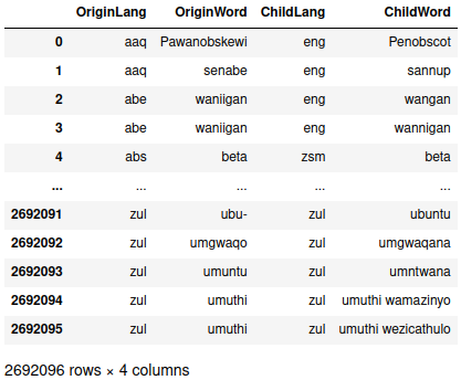

Since there were multiple ways to specify the relationship before, we deduplicated the rows so the redundancies don’t artificially inflate the relationships between languages. That leaves around 2.7 million entries in the data, but I’m only interested in the raw counts of a word in one language being the ancestor of another, so a group-and-count operation is warranted.

> etymology_count = etymology_info.groupby(["OriginLang", "ChildLang"]).count()
> etymology_count = etymology_count["OriginWord"].reset_index().rename(columns={"OriginWord": "Count"})
> etymology_count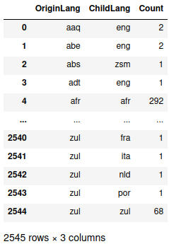

There are 2,545 unique origin-child relationships in the data, but several combinations in the head and the tail have only one or two instances. If we bin the results, we see that only a relative few seem to be major relationships:

> pd.cut(etymology_count["Count"], bins=[0,5,10,50,100,500,1000,1e10]).value_counts()
(0.0, 5.0]                 1593
(10.0, 50.0]                367
(5.0, 10.0]                 243
(100.0, 500.0]              139
(50.0, 100.0]                91
(1000.0, 10000000000.0]      71
(500.0, 1000.0]              41
Name: Count, dtype: int64
> 
> etymology_count["Count"].max()
613775

Around one-tenth of the relationships have more than 50 entries, at least some of which are fairly extreme. It looks like those extreme values are mainly when the origin and child languages are the same:

> etymology_count.loc[etymology_count["Count"] > 10000, :]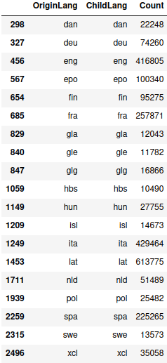

I’m only interested in the relationships between langauges, not relationships within a language, so I just drop all of those and take another look:

> etymology_count = etymology_count.loc[etymology_count["OriginLang"] != etymology_count["ChildLang"], :]
> pd.cut(etymology_count["Count"], bins=[0,5,10,50,100,500,1000,1e10]).value_counts()
(0.0, 5.0]                 1551
(10.0, 50.0]                333
(5.0, 10.0]                 226
(100.0, 500.0]              106
(50.0, 100.0]                80
(500.0, 1000.0]              22
(1000.0, 10000000000.0]      20
Name: Count, dtype: int64
>
> etymology_count["Count"].max()
6663

We’re now down to 2,338 relationships, the most common of which is several thousand entries. The vast bulk of the entries are still fairly few in number, with only about a quarter of the relationships existing in more than 50 word pairs. Additionally, we still have most of the languages present in the data:

> len(set(etymology_count["OriginLang"]).union(set(etymology_count["ChildLang"])))
386

Trying to plot this would still be too busy, so I decided to trim it down some more. Some experimentation showed that restricting the data to relationships with more than 500 entries gives us only 43 nodes, which is small enough that it should work okay.

> major_contributors = etymology_count.loc[etymology_count["Count"] > 500,:].copy()
> len(set(major_contributors["OriginLang"]).union(set(major_contributors["ChildLang"])))
43

Making the Graph

Since the data we’re trying to plot is represented as a series of one-way relationships with some size of interest, we want a weighted directed graph to contain it. Fortunately, the networkx package can read in a graph directly from a pandas dataframe, so no more transformation is needed.

import networkx as nx
from matplotlib.collections import PatchCollection
import matplotlib.pyplot as plt
plt.rcParams["figure.figsize"] = [9,7]

word_graph = nx.from_pandas_edgelist(major_contributors,
                                     source="OriginLang",
                                     target="ChildLang",
                                     edge_attr="Count",
                                     create_using=nx.DiGraph)

Then comes drawing the graph. I based the function largely off of an example from the networkx documentation. (Note that I experimented for a while to find a good layout for the nodes in the plot; while kamada_kawai_layout isn’t great for the full graph, it seemed better than the other ones that I tried.)

> def draw_word_graph(word_graph):
>     """
>     Draws a graph of the relationships between words in a graph.  Uses
>     kamada_kawai_layout as, while no layouts were particularly good, this one
>     was the best of the lot.
>     """
>     positions = nx.kamada_kawai_layout(word_graph)
>     edge_colors = [v for k,v in nx.get_edge_attributes(word_graph, "Count").items()]
>     
>     # if you want the nodes drawn, use nx.draw_networkx_nodes; I was fine
>     # with just the language codes in this case
>     edges = nx.draw_networkx_edges(word_graph, pos=positions,
>                                    edge_color=edge_colors,
>                                    edge_cmap=plt.cm.magma)
>     labels = nx.draw_networkx_labels(word_graph, pos=positions)
> 
>     # this code block only contributes a legend bar on the left; leave it out
>     # if you don't want that
>     pc = PatchCollection(edges, cmap=plt.cm.magma)
>     pc.set_array(edge_colors)
>     plt.colorbar(pc)
> 
>     ax = plt.gca()
>     ax.set_axis_off()
>     plt.show()
> 
> draw_word_graph(word_graph)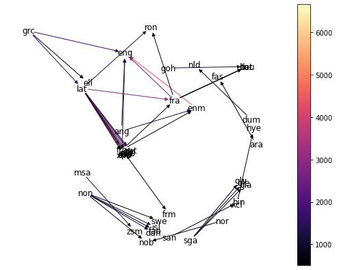

It’s a bit cluttered, but some things that can be seen in the above graph are:

• lat (Latin) is the parent of words in quite a few different languages. It doesn’t have any direct link to eng (modern English), though.
• ron (Romanian) only seems to have strong heritage from lat and fra (French).
• non (Old Norse) has a lot of words which turn up in modern-day neighbors nob (Bokmål, one of the written standards for modern Norwegian), swe (Swedish), and dan (Danish).
• Other langauges without ancestors in this data include msa (Malay), goh (Old High German), dum (Middle Dutch), and san (Sanskrit).

Out of curiosity, let’s zoom in a bit on English’s ancestors. Conveniently, networkx does have a function for getting all ancestors of a node in a directed graph, so that’s easy to accomplish.

> # .predecessors() gets ONLY the predecessors, so "eng" has to be manually
> # added to the node set
> english_ancestors = word_graph.predecessors("eng")
> english_graph = word_graph.subgraph(list(english_ancestors) + ["eng"])
> draw_word_graph(english_graph)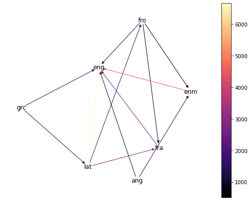

The most prominent direct ancestor of modern English is, perhaps predictably, Middle English (enm), though we also have plenty of words with Ancient Greek (grc), Old French (fro), modern French, and Old English (ang) heritage.