Detecting Streaks in R
Inspired by this post, which tries to calculate streaks in Python’s pandas library, I thought I’d give it a try in R, since it’s all just dataframe operations in the Python post. I won’t repeat his analysis, but I will replicate the streak determination and some of the plots. The data he uses is here.
Determining Streaks
As outlined in the above post, we first need a little dummy data to play with. For reproducability’s sake, I’m just using a fixed vector.
> library(tidyverse)
> x <- data.frame(trials=c(0,1,1,1,0,0,1,0,1,1,1,0,0,0,0,0,1))
The start of a streak is indicated when the two consecutive values are different. We have to handle this a little differently than in Python, though. The lag() function from dplyr generates an NA as the first value in the lagged vector, and comparisons involving NA will return NA:
> x <- x %>% mutate(lagged = lag(trials)) %>%  #note: that's dplyr::lag, not stats::lag
        mutate(start = (trials != lagged))
> x
   trials lagged start
1       0     NA    NA
2       1      0  TRUE
3       1      1 FALSE
4       1      1 FALSE
5       0      1  TRUE
6       0      0 FALSE
7       1      0  TRUE
8       0      1  TRUE
9       1      0  TRUE
10      1      1 FALSE
11      1      1 FALSE
12      0      1  TRUE
13      0      0 FALSE
14      0      0 FALSE
15      0      0 FALSE
16      0      0 FALSE
17      1      0  TRUE
Since we know that the first entry will always be the start of a streak, we can fix this by just setting the first element to TRUE:
> x[1, "start"] <- TRUEFrom there, we can get a little clever. Like in the Python post, R will happily convert booleans to numerics if prompted, so we can come up with an identification of when a streak starts by taking a cumulative sum of the start column:
> x <- x %>% mutate(streak_id = cumsum(start))
> x
   trials lagged start streak_id
1       0     NA  TRUE         1
2       1      0  TRUE         2
3       1      1 FALSE         2
4       1      1 FALSE         2
5       0      1  TRUE         3
6       0      0 FALSE         3
7       1      0  TRUE         4
8       0      1  TRUE         5
9       1      0  TRUE         6
10      1      1 FALSE         6
11      1      1 FALSE         6
12      0      1  TRUE         7
13      0      0 FALSE         7
14      0      0 FALSE         7
15      0      0 FALSE         7
16      0      0 FALSE         7
17      1      0  TRUE         8
From there, we just group by streak_id, get the row number for each row in each group, and then ungroup to get our final result. One convenient thing in this case is that R is one-indexed, so we don’t have to add 1 to the streak counter like in Python.
> x <- x %>% group_by(streak_id) %>% mutate(streak = row_number()) %>% ungroup()
> x
# A tibble: 17 x 5
   trials lagged start streak_id streak
    <dbl>  <dbl> <lgl>     <int>  <int>
 1      0     NA TRUE          1      1
 2      1      0 TRUE          2      1
 3      1      1 FALSE         2      2
 4      1      1 FALSE         2      3
 5      0      1 TRUE          3      1
 6      0      0 FALSE         3      2
 7      1      0 TRUE          4      1
 8      0      1 TRUE          5      1
 9      1      0 TRUE          6      1
10      1      1 FALSE         6      2
11      1      1 FALSE         6      3
12      0      1 TRUE          7      1
13      0      0 FALSE         7      2
14      0      0 FALSE         7      3
15      0      0 FALSE         7      4
16      0      0 FALSE         7      5
17      1      0 TRUE          8      1
Bringing this all together into one function:
get_streaks <- function(vec){
    x <- data.frame(trials=vec)
    x <- x %>% mutate(lagged=lag(trials)) %>%  #note: that's dplyr::lag, not stats::lag
            mutate(start=(trials != lagged))
    x[1, "start"] <- TRUE
    x <- x %>% mutate(streak_id=cumsum(start))
    x <- x %>% group_by(streak_id) %>% mutate(streak=row_number()) %>%
        ungroup()
    return(x)
}
Plotting Streaks
Replicating the initial plot is pretty quick:
> shots <- read_csv("playoff_shots.csv")
> durant_ft <- shots %>% filter(player_name == "Kevin Durant" & shot_type == "FT")
> durant_ft <- get_streaks(durant_ft$result)

> ggplot(durant_ft, aes(x=1:nrow(durant_ft), y=streak)) + geom_bar(stat="identity")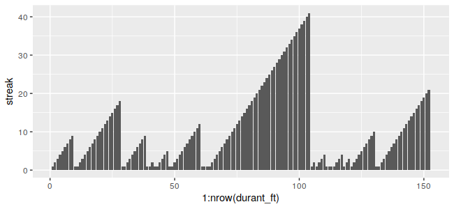
Recreating one of the later ones requires additional work, but ggplot2 has all of the necessary functionality on its own, so we don’t need to bring in anything to extend it, it’s just lengthy. We also make the slight tweak to the streak variable so that the miss streaks go down under the x=0 axis.
> durant_ft2 <- durant_ft %>% mutate(streak = streak * ifelse(trials == "make", 1, -1))
> caption <- paste(c("Kevin Durant", "FT"), collapse = "\n")
> ggplot(durant_ft2, aes(x=1:nrow(durant_ft2), y=streak)) +
>     geom_bar(aes(fill=trials), stat="identity") +
>     theme_void() +
>     geom_hline(yintercept = 0) +
>     geom_vline(xintercept = 0) +
>     scale_fill_manual(values=c("make"="darkgreen", "miss"="red"), guide=FALSE) +
>     annotate(geom="text", label=caption, x=nrow(durant_ft2), y=max(durant_ft2$streak),
>              hjust="right", vjust="top")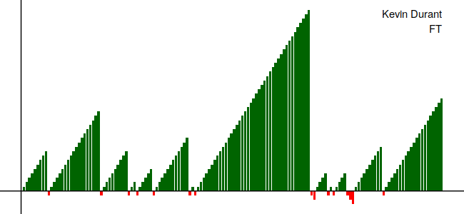
Full code for this post is available here.