A Slightly More Advanced MCMC Example
I’ve seen a number of examples of MCMC algorithms, and while they’re all solid, a lot of them tend to be a bit too neat - they have a fairly simple model, a single predictor (maybe two), and not much else. This one is a good example, as it covers the theory in detail, but it’s using an obviously toy data set. So I decided to throw together a slightly more intricate example, highlighting a couple of issues and tricks worth noting for a handwritten implementation.
Note that this post is written under the assumption that the reader already has some knowledge about what MCMC is generally for and broadly how it works. This post is all R code (see here), with no JAGS or BUGS or such. The tidyverse, patchwork, and ISLR libraries are required – the former two for the plots, the latter for the data set used.
Overview & Data Prep
We’ll use the Default data set from the ISLR package, which supplies a yes/no column for the whether someone defaulted (which is what we’ll be predicting) and three variables describing whether or not they’re a student, their account balance, and their annual income (which will be our predictors). Since this is a binary classification problem, logistic regression will work fine here. Using logistic regression also means that we can train a GLM and check our results against the GLM output.
As for the data itself, the only transformations necessary to get started are for the default and student variables, which are character columns with values of “yes” and “no” in the unmodified dataframe. We need those to be numerics with values of 0 or 1, which correspond to “no” and “yes” respectively in this case.
> data(Default, package="ISLR")
> Def2 <- Default %>%
>     mutate(default = as.integer(as.character(default) == "Yes")) %>%
>     mutate(student = as.integer(as.character(student) == "Yes"))
MCMC Functions
MCMC, as a Bayesian method, comes down to working with priors and likelihoods. For the priors on the coefficients, we’re using generic, uninformative normal distributions, with mean 0 and variance 100.
> prior <- function(betas){
>     return(prod(sapply(betas, dnorm, mean=0, sd=10)))
> }
Since our outcome is binary, our likelihood density is a Bernoulli distribution:
$$f(p) = p^y (1-p)^{1-y}$$
But the probability is a function of the predictors and the coefficients we’re modeling, so \(p\) isn’t constant. Instead, the probability is calculated via the expit function:
$$ p = \frac{e^{X\beta}}{1 + e^{X\beta}} $$
where \(X\) is the matrix of predictors and \(\beta\) is the vector of model coefficients.
> likelihood <- function(X, y, betas){
>     e <- exp(X %*% betas)
>     px <- e/(1+e)
>     return(px^y * ((1-px)^(1-y)))
> }
Our “posterior” is just the product of these two (it’s not technically the posterior since we need to divide by an appropriate marginal distribution, but that cancels out of the math so we don’t need to calculate it):
> log_posterior <- function(X, y, betas){
>     log_prior <- log(prior(betas))
>     log_likelihoods <- log(likelihood(X, y, betas))
>     return(log_prior + sum(log_likelihoods))
> }
Note that we’re actually calculating the log of the posterior. This is done as a protection against underflow errors – we’re multiplying together 10,000 numbers between 0 and 1, which makes it easy for the product to get small enough for R to simply declare that it’s zero, which will ruin the computation.
From there, then, we’re implementing standard Metropolis-Hastings:
- Start with initial values for the coefficients we’re looking for.
- Perturb the values slightly.
- Calculate the acceptance ratio (or rejection ratio - I’ve heard it both ways, and the code uses the latter term) for each new value
- Accept or reject each new value individually, comparing them to the random draws from a Uniform(0,1) distribution (or the log of the draw, in this case).
- Repeat from step 2 for a specified number of times.
MCMC <- function(X, y, n, beta_start=c(0,0,0,0), jump_dist_sd=0.1){
>     B <- ncol(X)   # number of betas (coefficients)
>     beta <- matrix(nrow=n, ncol=B)
>     beta[1,] <- beta_start
>     for(i in 2:n){
>         current_betas <- beta[i-1,]
>         new_betas <- current_betas + rnorm(B, mean=0, sd=jump_dist_sd)
>         for(j in 1:B){
>             test_betas <- current_betas
>             test_betas[j] <- new_betas[j]
>             rr <- log_posterior(X, y, test_betas) - log_posterior(X, y, current_betas)
>             if(log(runif(1)) < rr){
>                 beta[i,j] <- new_betas[j]
>             } else {
>                 beta[i,j] <- current_betas[j]
>             }
>         }
>     }
>     return(beta)
> }
I made a couple of attempts at trying to improve the speed of the update operation. One was to move the inner for loop to its own function and use sapply() to see if that was faster, but it was about the same speed as the for loop (10,000 updates in about 43 seconds on my machine). I also tried parallelizing the update process with the parallel package, but that was quite a bit slower (10,000 updates in about 350 seconds). Since each update operation is pretty quick to begin with, it looks like the overhead in parallelizing it outweighs any gains by a lot.
Running MCMC
Running it in this form immediately throws an error:
{MCMC code & error}
> set.seed(1000)
> burn_in_length <- 10000
> N <- 50000   # total number of points
>
> y <- Def2$default
> X <- cbind(1, as.matrix(Def2[,2:4]))   # pad with a column of ones for intercept
>
> beta <- MCMC(X, y, n=N, jump_dist_sd=0.05)
Error in if (log(runif(1)) < rr) { :
  missing value where TRUE/FALSE needed
A little bit of hunting reveals the culprit: scaling. We’re currently changing the values of our parameters by adding a random value from a normal distribution with mean 0 and standard deviation 0.05. If you look at the data, however…
> head(Def2)
  default student   balance    income
1       0       0  729.5265 44361.625
2       0       1  817.1804 12106.135
3       0       0 1073.5492 31767.139
4       0       0  529.2506 35704.494
5       0       0  785.6559 38463.496
6       0       1  919.5885  7491.559
If the coefficient for income becomes 0.005 – a tenth of a standard deviation in the jumping distribution – and all others are zero, then the likelihood function for that first row involves computing roughly \(e^{2200}\), which is somewhere over \(10^{950}\). A little testing will show that R starts returning Inf around \(e^{710}\). And while R seems okay with comparing a real number and Inf, calculating the rejection ratio required taking the difference between two infinities, and that’s where R returns NaN.
I’m unsure of what the best way to solve this is, and I don’t recall how JAGS or BUGS do this, but the simplest solution is just rescaling the variables to something less extreme:
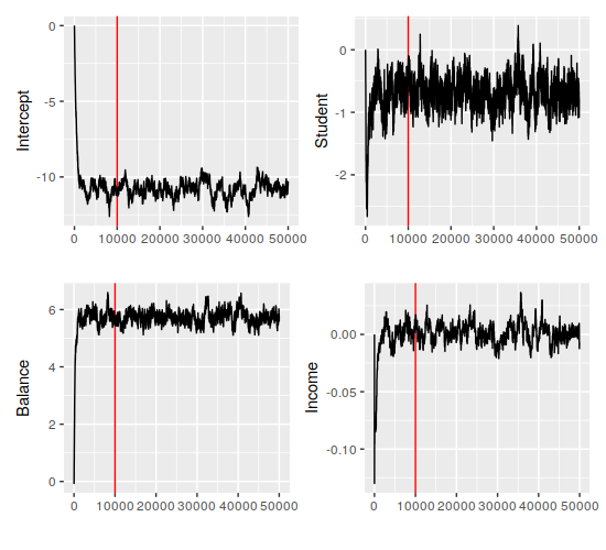
> Def2 <- Def2 %>% mutate(balance=balance/1000) %>% mutate(income=income/1000)The MCMC code runs just fine after this, which means we can look at the coefficients that we’ve gotten (red lines indicate the end of the burn-in period):

This looks pretty stable, actually – all four parameters have settled in their ranges comfortably before the burn-in period ended. Additionally, it looks like everything but the income coefficient is clearly nonzero. The quantiles back that up (the first row is the means):
> MCMC_results <- apply(beta, MARGIN=2, function(x){c(mean(x), quantile(x, c(0.025, 0.5, 0.975)))})
> colnames(MCMC_results) <- c("Intercept", "student", "balance", "income")
> round(MCMC_results, 4)
      Intercept student balance  income
       -10.7973 -0.6790  5.7285  0.0015
2.5%   -11.8710 -1.1226  5.3091 -0.0142
50%    -10.7834 -0.6837  5.7256  0.0015
97.5%   -9.8218 -0.1978  6.2304  0.0184
Comparison
Of course, if we can’t find some way to confirm whether we’ve coded this up right, we can’t be sure that the model is giving sensible results. This CrossValidated post talks about a couple, but in this case, we can just run R’s glm() function on the data and see if it matches. Fortunately, it does:
> glm_model <- glm(default ~ student + balance + income, data=Def2, family=binomial(link="logit"))
> summary(glm_model)  # only posting an excerpt of the output for brevity
Coefficients:
              Estimate Std. Error z value Pr(>|z|)
(Intercept) -10.869045   0.492256 -22.080  < 2e-16 ***
student      -0.646776   0.236253  -2.738  0.00619 **
balance       5.736505   0.231895  24.738  < 2e-16 ***
income        0.003033   0.008203   0.370  0.71152
---
Signif. codes:  0 ‘***’ 0.001 ‘**’ 0.01 ‘*’ 0.05 ‘.’ 0.1 ‘ ’ 1
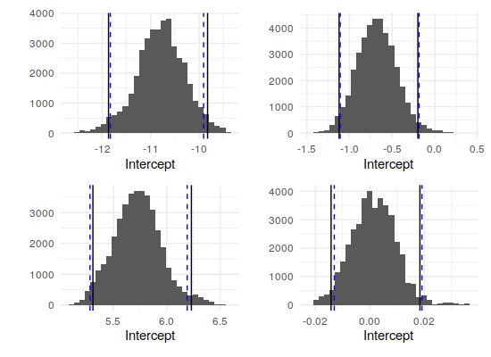
As one final comparison, we can look at the distribution of the MCMC samples (after the burn-in period), overlaid with the 95% interval from the samples' quantiles (black lines) and the 95% confidence interval from the GLM model (dashed blue lines):
