PySpark + MySQL Tutorial

This post is meant as a short tutorial on how to set up PySpark to access a MySQL database and run a quick machine learning algorithm with it. Both PySpark and MySQL are locally installed onto a computer running Kubuntu 20.04 in this example, so this can be done without any external resources.

Requirements

Installing MySQL onto a Linux machine is fairly quick thanks to the apt package manager:

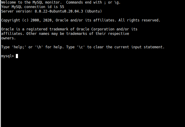
sudo apt install mysql-server

Once it’s installed, you can run sudo mysql in a terminal to access MySQL from the command line:

For Spark, just running pip install pyspark will install Spark as well as the Python interface. For this example, I’m also using mysql-connector-python and pandas to transfer the data from CSV files into the MySQL database. Spark can load CSV files directly, but that won’t be used for the sake of this example.

Finally, we need the Java drivers that will let Spark connect to MySQL. I didn’t see a good way to install them through apt, so I downloaded the driver from the MySQL website and installed it manually. You may need the location of the driver file later on, depending on where it was installed, so finding it may be necessary. On Kubuntu, the driver file was installed to “/usr/share/java/”.

The data that I’m using is the wine quality dataset from the UCI machine learning repository. It’s not especially large, with only around 6500 examples total, but it’s clean and easy to use for this example. There are a few possible ways to use it for machine learning or other predictive purposes, but I’m going to focus on predicting whether the wine in question is red or white.

Writing Data to MySQL

The first step is to read in the data. The only things worth noting here are that the files are semicolon-delimited, and we need to create the column for whether a wine is white or red ourselves:

import pandas as pd

red_wines = pd.read_csv("winequality-red.csv", sep=";")
red_wines["is_red"] = 1
white_wines = pd.read_csv("winequality-white.csv", sep=";")
white_wines["is_red"] = 0
all_wines = pd.concat([red_wines, white_wines])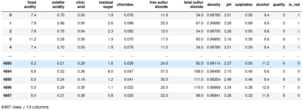

MySQL is similarly straightforward as you just set up the new database and an appropriate table. You will need to ensure that your user has privileges to edit the table, though; if you need to change privileges, that will have to be done from the MySQL prompt.

import mysql.connector

db_connection = mysql.connector.connect(user="me", password="me")
db_cursor = db_connection.cursor()
db_cursor.execute("CREATE DATABASE TestDB;")
db_cursor.execute("USE TestDB;")

db_cursor.execute("CREATE TABLE Wines(fixed_acidity FLOAT, volatile_acidity FLOAT, \
                   citric_acid FLOAT, residual_sugar FLOAT, chlorides FLOAT, \
                   free_so2 FLOAT, total_so2 FLOAT, density FLOAT, pH FLOAT, \
                   sulphates FLOAT, alcohol FLOAT, quality INT, is_red INT);")

And then load the data. MySQL can load multiple rows into a table at once if the contents of each row are contained within parentheses and comma-delimited like this:

wine_tuples = list(all_wines.itertuples(index=False, name=None))
wine_tuples_string = ",".join(["(" + ",".join([str(w) for w in wt]) + ")" for wt in wine_tuples])
wine_tuples_string[:100]
## '(7.4,0.7,0.0,1.9,0.076,11.0,34.0,0.9978,3.51,0.56,9.4,5,1),(7.8,0.88,0.0,2.6,0.098,25.0,67.0,0.9968,'

And then upload into the database. The FLUSH TABLES command is used to get the database to actually update the table with the rows, otherwise the changes are merely staged and would eventually be discarded once the connection was closed.

db_cursor.execute("INSERT INTO Wines(fixed_acidity, volatile_acidity, citric_acid,\
                   residual_sugar, chlorides, free_so2, total_so2, density, pH,\
                   sulphates, alcohol, quality, is_red) VALUES " + wine_tuples_string + ";")
db_cursor.execute("FLUSH TABLES;")

Accessing MySQL with PySpark

Starting a Spark session from Python is fairly straightforward. Again, I had to specify the location of the MySQL Java driver, which is the only subtlety that I found. Loading the table afterward is similarly simple, despite the number of options that need to be specified, though you’ll need the port number that MySQL is on when loading the data from the database (the default port is 3306).

from pyspark.sql import SparkSession
spark = SparkSession.builder.config("spark.jars", "/usr/share/java/mysql-connector-java-8.0.22.jar") \
    .master("local").appName("PySpark_MySQL_test").getOrCreate()

wine_df = spark.read.format("jdbc").option("url", "jdbc:mysql://localhost:3306/TestDB") \
    .option("driver", "com.mysql.jdbc.Driver").option("dbtable", "Wines") \
    .option("user", "me").option("password", "me").load()

If you’re loading data into Spark from a file, you’ll probably want to specify a schema to avoid making Spark infer it. For a MySQL database, however, that’s not necessary since it has its own schema and Spark can translate it.

Training the Model

Finally, training the model. As always, split the train and test data first:

train_df, test_df = wine_df.randomSplit([.8, .2], seed=12345)

Specifying the model can be done a few ways, including the ability to use an R-like formula to specify the model. Here I’ll use the VectorAssembler, which basically just concatenates all the features into a single list:

from pyspark.ml.feature import VectorAssembler

predictors = ["fixed_acidity", "volatile_acidity", "citric_acid", "residual_sugar", "chlorides",
              "free_so2", "total_so2", "density", "pH", "sulphates", "alcohol"]
vec_assembler = VectorAssembler(inputCols=predictors, outputCol="features")
vec_train_df = vec_assembler.transform(train_df)
vec_train_df.select("features", "is_red").show(5)

## +--------------------+------+
## |            features|is_red|
## +--------------------+------+
## |[3.8,0.31,0.02,11...|     0|
## |[3.9,0.225,0.4,4....|     0|
## |[4.2,0.17,0.36,1....|     0|
## |[4.2,0.215,0.23,5...|     0|
## |[4.4,0.32,0.39,4....|     0|
## +--------------------+------+
## only showing top 5 rows

Then a logistic regression model can be trained on the data:

from pyspark.ml.classification import LogisticRegression

lr = LogisticRegression(labelCol="is_red", featuresCol="features")
lr_model = lr.fit(vec_train_df)

And we can get the predictions that the model makes for the test data.

vec_test_df = vec_assembler.transform(test_df)
predictions = lr_model.transform(vec_test_df)

PySpark also has a Pipeline class, which can intelligently connect up all of the separate steps into a single operation, if you prefer:

from pyspark.ml import Pipeline
pipeline = Pipeline(stages=[vec_assembler, lr])
pipeline_model = pipeline.fit(train_df)
predictions = pipeline_model.transform(test_df)

Regardless, evaluating the model is necessary. Spark seems a little limited in the native options for evaluating models - the BinaryClassificationEvaluator below only seems to support area under the curve for ROC (default) or the precision-recall curve.

from pyspark.ml.evaluation import BinaryClassificationEvaluator
evaluator = BinaryClassificationEvaluator(labelCol="is_red")
evaluator.evaluate(predictions)
## 0.9917049465379387

Note that the logistic regression model will actually return three columns of prediction data:

• rawPrediction depends on the model used, but here refers to the value of the linear part of the logistic regression model before being transformed
• probability is an array of the actual probabilities for each class
• prediction is the actual class prediction

predictions.select("rawPrediction", "probability", "prediction").toPandas().head()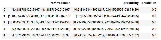

As shown above, the toPandas() method to return the prediction data as a pandas dataframe, so other metrics are possible to calculate with either pandas or numpy.

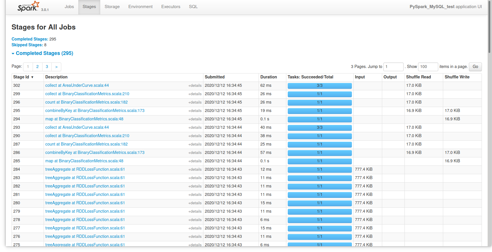
Finally, if you want to look at an overview of Spark’s activity during the session, you can open a browser tab to localhost:4040 and see an overview of it: