LDA vs QDA vs Logistic Regression
There are plenty of methods to choose from for classification problems, all with their own strengths and weaknesses. This post will try to compare three of the more basic ones: linear discriminant analysis (LDA), quadratic discriminant analysis (QDA), and logistic regression.
Theory: LDA and QDA
Both LDA and QDA result from the same ideas, apart from one different assumption. To start with, consider Bayes' theorem, where we’re trying to find the probability of a datum \(x\) belonging to one of \(K\) classes \(k\), and each class has their own probability density function \(f_k\) and prior probability \(\pi_k\):
$$ P(k| X=x) = \frac{f_k(x) \pi_k}{\sum_{l=1}^K f_l(x) \pi_l} $$
For the individual discriminant functions, comparing the likelihood of two classes \(k\) and \(l\) can be accomplished by looking at the log of the ratio of the posteriors:
$$ \log\left(\frac{P(k | X=x)}{P(l| X=x)}\right) = \log\frac{f_k(x)}{f_l(x)} + \log\frac{\pi_k}{\pi_l} $$
This leaves the question of what densities \(f_k\) to use. We can model each class density with a multivariate normal distribution with mean vector \(\mu_k\) and covariance matrix \(\boldsymbol\Sigma_k\):
$$ f_k(x) = \frac{1}{(2\pi)^{p/2} |\boldsymbol\Sigma_k|^{1/2}} \exp\left( -\frac{1}{2}(x - \mu_k)^T \boldsymbol\Sigma_k^{-1}(x-\mu_k) \right) $$
If you assume that all of the covariance matrices are the same – \(\boldsymbol\Sigma_k = \boldsymbol\Sigma\) for all \(k\) – then for two classes,
$$ \log\left(\frac{P(G=k | X=x)}{P(G=l | X=x)}\right) = \log\frac{\pi_k}{\pi_l} - \frac{1}{2}(x - \mu_k)^T \boldsymbol\Sigma^{-1}(x-\mu_k) + x^T \boldsymbol\Sigma^{-1}(\mu_k - \mu_l) $$
For three or more classes, this generalizes to finding the class \(k\) such that
$$ \delta_k(x) = \log \pi_k + x^T \boldsymbol\Sigma^{-1} \mu_k - \frac{1}{2} \mu_k^T \boldsymbol\Sigma^{-1}\mu_k $$
is maximized. This is our discriminant, which is linear in the sense that it has only a linear dependence on \(x\) – hence the name LDA. If, instead, you choose to keep the individual covariance matrices different, then the discriminant function becomes
$$ \delta_k(x) = \log\pi_k - \frac{1}{2} \log |\boldsymbol\Sigma_k| - \frac{1}{2}(x-\mu_k)^T\boldsymbol\Sigma_k^{-1}(x-\mu_k) $$
which is quadratic in \(x\) in the last term, hence QDA. Since QDA allows for differences between covariance matrices, it should never be less flexible than LDA. That said, QDA does require many more parameters because of the multiple covariance matrices to store, with the total number of parameters roughly scaling with \(Kp^2\). Whether that extra flexibility is useful for prediction or a potential source of overfitting will depend on the situation, though Occam’s razor would suggest that the simpler model of LDA will suffice unless the covariance differences between classes are significant.
There are plenty of other variants on these methods – an interesting one is regularized discriminant analysis, which tries to shrink the individual covariance matrices in QDA towards a single common one like in LDA. However, these variants are beyond the scope of this post.
Theory: Logistic Regression
Returning to the log of the ratio of posteriors for a moment, suppose we wanted to model the results of that log ratio as a linear function of \(x\). Letting class \(K\) be the reference class, we have
$$ \log\left(\frac{P(k | X=x)}{P(K | X=x)}\right) = \beta_{0k} + \beta_{k}^Tx $$
for each of the other \(K-1\) classes. We can transform these into probabilities for each class – for classes 1 to \(K-1\),
$$ P(k | X=x) = \frac{\exp(\beta_{0k} + \beta_{k}^Tx)}{1 + \sum_{l=1}^{K-1} \exp(\beta_{0k} + \beta_{k}^Tx)} $$
and for class \(K\),
$$ P(K | X=x) = \frac{1}{1 + \sum_{l=1}^{K-1} \exp(\beta_{0k} + \beta_{k}^Tx)} $$
Logistic regression has acouple of advantages over LDA and QDA. Since we’re not making any assumptions about the distribution of \(x\), logistic regression should (in theory) be able to model data that includes non-normal features much better than LDA and QDA. Logistic regression also seems more suited towards exploratory analyses, as the regression coefficients in the model have clear interpretations: the change in the log-odds per unit change in the features.
On the other hand, producing the best estimates for the \(\beta_k\) coefficients in logistic regression has to be done with some iterative updating algorithm, while LDA and QDA just need some covariance calculations and basic matrix operations. The algorithm generally converges pretty well, though I have seen cases where attempting a logistic regression fit will cause an error or warning about convergence if there’s some issue with the data.
Model 1: Palmer’s Penguins Data
The easiest way to try and highlight the differences between the methods is to simply use them on a few models. First is the Palmer’s Penguins data, a recent alternative of sorts to the iris dataset with a purpose. For this quick model, we’re just predicting the species from four numeric features: bill length, bill depth, flipper length, and body mass.
library(tidyverse)
library(caret)
# additional requirements: MASS, nnet

penguins <- read.csv("https://raw.githubusercontent.com/rfordatascience/tidytuesday/master/data/2020/2020-07-28/penguins.csv")

penguin_measurements <- penguins %>%
    select(species, bill_length_mm, bill_depth_mm, flipper_length_mm, body_mass_g) %>%
    drop_na()
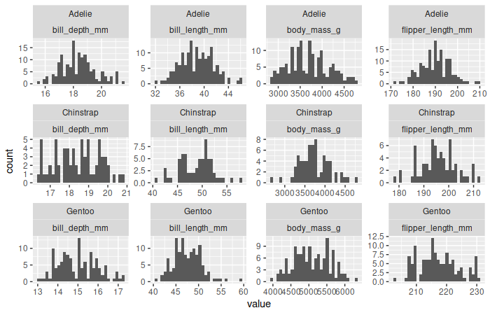
Testing for multivariate normality is a tricky thing. Checking whether the individual variables are normally distributed is not sufficient by itself to prove multivariate normality, even if it looks reasonable like it does here:

It requires its own tests – a recent review of several methods can be found here. Some tests can be found in the MVN library, and one is employed here:
library(MVN)
Adelie <- penguin_measurements %>% filter(species=="Adelie") %>% select(-species)
Chinstrap <- penguin_measurements %>% filter(species=="Chinstrap") %>% select(-species)
Gentoo <- penguin_measurements %>% filter(species=="Gentoo") %>% select(-species)
mvn(Adelie, mvnTest="energy")$multivariateNormality
##          Test Statistic p value MVN
## 1 E-statistic  1.118965    0.11 YES
mvn(Chinstrap, mvnTest="energy")$multivariateNormality
##          Test Statistic p value MVN
## 1 E-statistic  1.050637   0.273 YES
mvn(Gentoo, mvnTest="energy")$multivariateNormality
##          Test Statistic p value MVN
## 1 E-statistic  1.255741   0.018  NO
So two species of pengiuns seem to have their measurements be multivariate normal, though the third does not. But it will probably still work for the discriminant methods. (Both the MASS and nnet libraries must be installed,though they don’t have to be loaded – the former has the methods for LDA and QDA to use with caret, and the latter handles the multiclass logistic (multinomial) regression.)
lda_penguins <- train(data=penguin_measurements, species ~ ., method="lda",
                      trControl=trainControl(method="cv", number=10))
qda_penguins <- train(data=penguin_measurements, species ~ ., method="qda",
                      trControl=trainControl(method="cv", number=10))
logistic_penguins <- train(data=penguin_measurements, species ~ ., method="multinom",
                           trControl=trainControl(method="cv", number=10))

lda_penguins$results
##   parameter  Accuracy     Kappa AccuracySD    KappaSD
## 1      none 0.9855415 0.9772772 0.01524839 0.02395827
qda_penguins$results
##  parameter  Accuracy     Kappa AccuracySD    KappaSD
## 1      none 0.9855411 0.9771566 0.02440013 0.03843511
logistic_penguins$results
##  decay  Accuracy     Kappa AccuracySD    KappaSD
## 1 0e+00 0.9822638 0.9721749 0.02062338 0.03234243
## 2 1e-04 0.9822638 0.9721996 0.02485071 0.03884760
## 3 1e-01 0.9881462 0.9813075 0.01530539 0.02414735
All three models have similar and fairly high accuracies. (The three values for the logistic regression model arise because the nnet package trains it as a neural network, and there are three different weight decay rates that caret tries when fitting the model.)
Model 2: Wi-Fi Data
The second dataset is the Wireless Indoor Localization dataset, where 500 measurements of the strengths of seven different wi-fi signals are taken in each of four different rooms. The measurements are all integers, so they don’t follow a normal distribution particularly well:
wifi <- read.table("wifi_localization.txt")
mvn(wifi[wifi$V8==1, 1:7], mvnTest="energy")  #just for one class since the output is long
## $multivariateNormality
##          Test Statistic p value MVN
## 1 E-statistic  2.214773       0  NO
##
## $univariateNormality
##           Test  Variable Statistic   p value Normality
## 1 Shapiro-Wilk    V1        0.9775  <0.001      NO
## 2 Shapiro-Wilk    V2        0.9861   1e-04      NO
## 3 Shapiro-Wilk    V3        0.9916  0.0064      NO
## 4 Shapiro-Wilk    V4        0.9846  <0.001      NO
## 5 Shapiro-Wilk    V5        0.9735  <0.001      NO
## 6 Shapiro-Wilk    V6        0.9761  <0.001      NO
## 7 Shapiro-Wilk    V7        0.9863   1e-04      NO
But it turns out that the models are still fairly accurate.
lda_wifi <- train(data=wifi, as.factor(V8) ~ ., method="lda",
                  trControl=trainControl(method="cv", number=10))
qda_wifi <- train(data=wifi, as.factor(V8) ~ ., method="qda",
                  trControl=trainControl(method="cv", number=10))
logistic_wifi <- train(data=wifi, as.factor(V8) ~ ., method="multinom",
                       trControl=trainControl(method="cv", number=10))

lda_wifi$results
##   parameter Accuracy Kappa AccuracySD    KappaSD
## 1      none   0.9715 0.962 0.01055409 0.01407212
qda_wifi$results
##   parameter Accuracy Kappa  AccuracySD   KappaSD
## 1      none   0.9805 0.974 0.008644202 0.0115256
logistic_wifi$results
##   decay Accuracy     Kappa  AccuracySD    KappaSD
## 1 0e+00   0.9810 0.9746667 0.008096639 0.01079552
## 2 1e-04   0.9815 0.9753333 0.007835106 0.01044681
## 3 1e-01   0.9765 0.9686667 0.012483322 0.01664443
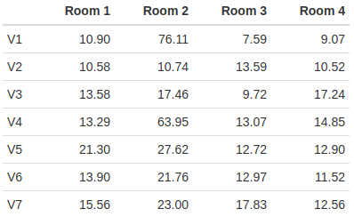
Since logistic regression doesn’t require normal data, it fares better than the other two. But what I want to point out here is that QDA is notably more accurate than LDA on this dataset. In this case, it comes from the fact that the covariance matrices are pretty dissimilar for the four rooms. Showing all four 7-by-7 covariance matrices isn’t practical here, but just the differences in the variances of the variables by class is pretty suggestive:

Model 3: Census Income Data
The third dataset is the Census Income dataset, which consists of about records extracted from the 1994 Census database and a two-level outcome factor for whether the person in question made over $50,000 per year or not. This one required a little more cleaning, mostly to filter out additional variables and condense the factor for education into something a little more compact:
adults <- read.csv("adult.data", header=FALSE, stringsAsFactors=TRUE)
names(adults) <- c("age", "workclass", "fnlwgt", "education", "education_num",
                   "marital_status", "occupation", "relationship", "race",
                   "sex", "capital_gain", "capital_loss", "hours_per_week",
                   "native_country", "salary")
adults <- adults %>%
    select(age, fnlwgt, education, sex, capital_gain, capital_loss, salary) %>%
    mutate(education=fct_collapse(education,
                                  NoHS=c(" 10th", " 11th", " 12th", " 1st-4th",
                                         " 5th-6th", " 7th-8th", " 9th", " Preschool"),
                                  Associates=c(" Assoc-acdm", " Assoc-voc"),
                                  Bachelors=" Bachelors", Doctorate=" Doctorate",
                                  Masters=" Masters", HSgrad=" HS-grad",
                                  ProfSchool=" Prof-school", SomeCollege=" Some-college"),
           capital_gain = 1*(capital_gain>0),
           capital_loss = 1*(capital_loss>0))

lda_adults <- train(data=adults, salary ~ ., method="lda",
                    trControl=trainControl(method="cv", number=10))
qda_adults <- train(data=adults, salary ~ ., method="qda",
                    trControl=trainControl(method="cv", number=10))
logistic_adults <- train(data=adults, salary ~ ., method="multinom",
                         trControl=trainControl(method="cv", number=10))

lda_adults$results
##   parameter  Accuracy     Kappa  AccuracySD    KappaSD
## 1      none 0.8084827 0.4027094 0.006854388 0.02113622
qda_adults$results
##   parameter  Accuracy     Kappa  AccuracySD    KappaSD
## 1      none 0.7888579 0.3678485 0.007552935 0.02022411
logistic_adults$results
##   decay  Accuracy     Kappa  AccuracySD    KappaSD
## 1 0e+00 0.8108778 0.4004223 0.004550319 0.01776870
## 2 1e-04 0.8108778 0.4004223 0.004550319 0.01776870
## 3 1e-01 0.8108778 0.4003578 0.004414290 0.01754893
Despite the fact that there were several factor variables present (which would be interpreted as a collection of one-hot variables within the model), the LDA model doesn’t do appreciably worse than the logistic regression model. The QDA model has a distinctly lower accuracy than the other two, though I’m not sure why.
A side note: I had intended to include another factor variable or two into the model, but attempting to train the QDA model resulted in warnings about rank deficiency so it wouldn’t train.
Conclusions
LDA and logistic regression are both strong methods in general. QDA is about as strong as the other two in general, but it doesn’t have any real advantage over LDA unless the covariances really are different, and the fact that it requires training many more parameters could lead to rank deficiency issues or other problems while constructing the model.
In theory, the requirements of multivariate normality would hinder the use of LDA and QDA, since guaranteeing multivariate normality is difficult and a lot of normality tests can react very strongly to occasional outliers. As with a lot of statistical methods that state they require normality, though, LDA and QDA are somewhat tolerant of non-normal data in practice.