An Example With accumulate()

As with most useful (collections of) libraries, the tidyverse has a lot to offer. One interesting bit that I found recently was the accumulate() function in the purrr library, which allows you to apply a function over a succession of values in a vector. This post is a quick example of its use, using linear regression models.

The documentation gives a fairly brief description of the function:

accumulate applies a function recursively over a list from the left, while accumulate_right applies the function from the right. Unlike reduce both functions keep the intermediate results.

The call to accumulate requires a list or atomic vector and a function with two input variables, the output of the previous iterations and the next element in the vector (in that order). The obvious uses for this function would be cumulative sums or products, though base R already has the cumsum() and cumprod() functions. You could also take advantage of R’s ability to accept strings as formulas and then use accumulate() to build a character vector of formulas, and then train a model on each one.

Regression Example

For regression models, forward selection is a process for iteratively building the model by seeing which variable improves the model the most, adding it to the model, and repeating until some condition is met. This improvement is usually based on \(p\)-values or an error metric, but a (naive) idea, assuming you had all numeric (i.e., non-factor) variables, might be to add variables in decreasing order of absolute correlation. (I know that this isn’t a good idea for a number of reasons, and I’m leaving out the kind of exporatory analysis that should be done, but let’s see what happens.)

We’ll use the Boston dataset from the MASS library, and try to predict the median housing value using several numeric columns (leaving out a couple variables that are indicators or only have a few discrete values). First we get the columns in order of largest to smallest correlation by magnitude:

> library(MASS)
> library(tidyverse)
> 
> data(Boston)
> 
> cols_to_use <- c("crim", "zn", "indus", "nox", "age", "dis", "tax", "ptratio", "black", "lstat")
> correlations <- cor(Boston[,c(cols_to_use, "medv")])[1:10,11]
> strongest_to_least_corr <- names(sort(abs(correlations), decreasing = TRUE))
> strongest_to_least_corr
[1] "lstat"   "ptratio" "indus"   "tax"     "nox"     "crim"    "age"     "zn"      "black"   "dis"

Then accumulate() can help build the right side of the formula strings pretty easily:

> predictor_strings <- accumulate(strongest_to_least_corr, function(a,b){paste(a,b,sep=" + ")})
> model_strings <- paste("medv ~", predictor_strings)
> model_strings
 [1] "medv ~ lstat"                                                              
 [2] "medv ~ lstat + ptratio"                                                    
 [3] "medv ~ lstat + ptratio + indus"                                            
 [4] "medv ~ lstat + ptratio + indus + tax"                                      
 [5] "medv ~ lstat + ptratio + indus + tax + nox"                                
 [6] "medv ~ lstat + ptratio + indus + tax + nox + crim"                         
 [7] "medv ~ lstat + ptratio + indus + tax + nox + crim + age"                   
 [8] "medv ~ lstat + ptratio + indus + tax + nox + crim + age + zn"              
 [9] "medv ~ lstat + ptratio + indus + tax + nox + crim + age + zn + black"      
[10] "medv ~ lstat + ptratio + indus + tax + nox + crim + age + zn + black + dis"

And then we train a linear regression for each model string and look at the \(R^2\), both adjusted and not:

> unadj_R2 <- numeric(10)
> adj_R2 <- numeric(10)
> 
> for(i in 1:10){
>     model <- lm(model_strings[i], data=Boston)
>     m <- summary(model)
>     unadj_R2[i] <- m$r.squared
>     adj_R2[i] <- m$adj.r.squared
> }
> 
> R2_data <- data.frame(NumPredictors=1:10, AdjR2=adj_R2, UnadjR2=unadj_R2)
> ggplot(data=R2_data, aes(x=NumPredictors)) + geom_line(aes(y=UnadjR2, color="Unadjusted")) +
>     geom_line(aes(y=AdjR2, color="Adjusted")) + xlab("# of predictors") + ylab("R^2") +
>     theme(legend.title = element_blank()) + scale_x_continuous(breaks = seq(1, 10, by = 1))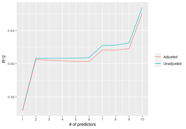

As noted above, this isn’t really a good idea, based on the adjusted \(R^2\) decreasing from two to six predictors, so there are clearly issues with the approach. But this is the kind of situation where accumulate() can provide much more concise code, which was the ultimate point.