Stock Correlation Versus LSTM Prediction Error

2020-09-19

When trying to look at examples of LSTMs in Keras, I’ve found a lot that focus on using them to predict stock prices in the future. Most are pretty bare-bones though, consisting of little more than a basic LSTM network and a quick plot of the prediction. Though I think the utility of these models is a little questionable, it brought a question into my head: how accurate are the predictions made by a model trained on one stock if it’s predicting on another stock?

The full code can be found here.

Problem Description

Stocks are correlated with each other to varying degrees, so the behaviors of any given pair of stocks may or may not track each other. The correlation between stocks is usually measured as the correlation of their returns (or at least, that’s what I’ve seen), and it’s easy to compute those yourself.

In addition, there are an immense number of posts and such about predicting stock prices with neural networks. These examples usually don’t go too deep, though, and they invariably train and check the model using data from the same stock. That’s reasonable enough, but it raises the question of how generalizable these models are. It doesn’t seem likely that the models would create good predictions if there was weak correlation between the stock they were trained on and the one it’s predicting on, but maybe it would work well enough for stocks that are more strongly correlated.

So the goal here is:

Get data on a large number of stocks (preferably hundreds).
Compute the correlations between the stocks.
Train an LSTM on a single, reference stock.
Make predictions for the other stocks using that LSTM model.
See how some error metric varies with correlation.

Getting the Data

Since I’m aiming to get data on a few hundred stocks, the first list that jumps to mind is the S&P 500. There are actually 505 tickers on there, but that’s because five of the companies have multiple share classes. I just discarded one class for each stock – the list I ended up using is in the GitHub repo for this post.

I downloaded the data from Tiingo via the pandas_datareader library. Tiingo limits free accounts to 500 unique symbols per month, so it’s feasible to grab this all at once, although you won’t to be able get data for any other ticker with that account for the remainder of the month.

import numpy as np
import pandas as pd
import pandas_datareader as pdr

with open("stock list.txt", "r") as f:
    stock_list = f.readlines()
stock_list = [s.strip().replace(".", "-") for s in stock_list]

stock_dfs = []
for i in range(50):
    # Tiingo can download multiple tickers per call, but just do 10 at a time to avoid abuse
    print(stock_list[10*i:10*(i+1)])
    stock_dfs.append(pdr.get_data_tiingo(stock_list[10*i:10*(i+1)], start="2000-01-01",
                                         api_key=TIINGO_API_KEY))

sp500_data = pd.concat(stock_dfs)

This will take several minutes to execute. If you’re running this code yourself, I recommend saving the data immediately afterward – the file that my run produced was almost 300 megabytes and contained about 2.3 million rows, so it’s not something you want to repeatedly download.

Selecting & Scaling Data

Since we’re dealing with an LSTM, we’d like to have data scaled down to a range that’s better handled by the LSTM inputs. And since the scales of the stocks differ, we need individual scalers for each stock. However, even though only the reference stock will have its data used for training, I want to ensure that all of the stocks have complete data for the same timeframe, since scaling the other stocks on just their test data would exaggerate how big some of the movements were in the stocks.

It turns out that complete data from 2001-01-01 to 2019-12-31 exists for 370 of the stocks, so I opted to just filter down to those.

adj_closes = sp500_data["adjClose"].unstack("symbol")
full_adj_closes = adj_closes.loc[(adj_closes.index < "2019-12-31"), :].dropna(axis=1)

It didn’t matter to me what the reference stock was, so I just picked one using random.choice() from Python’s standard library. The result was ALL (The Allstate Corporation), so we can set that as a constant, along with the lengths of the inputs and outputs for the network.

INPUT_LENGTH = 200
OUTPUT_LENGTH = 40
REFERENCE_STOCK = "ALL"

For scaling the data, most of the posts I saw used sklearn.preprocessing.MinMaxScaler() on the data to get it to a scale that the LSTM would work better with. I took it one step further, though – it seemed like monitoring the stock’s value changes in terms of percent change was a bit more consistent than using the absolute price. For example, if we consider the somewhat extreme case of Apple (AAPL):

import matplotlib.pyplot as plt

stock_data = full_adj_closes["AAPL"]
plt.subplot(2,1,1)
plt.plot(ALL_data.diff().values)
plt.ylabel("Absolute Change")

plt.subplot(2,1,2)
plt.plot(ALL_data.pct_change().values*100)
plt.xlabel("Date Index")
plt.ylabel("Percent Change")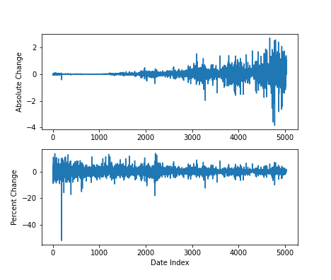

Image description.

To deal with this, I made a child class of the MinMaxScaler() which takes the logarithm of the data before applying the usual MinMaxScaler() functionality. As a result, percentage changes are now absolute changes.

from sklearn.preprocessing import MinMaxScaler

class LogMinMaxScaler(MinMaxScaler):
    """
    Essentially a modified version of the MinMaxScaler, where fitting
    the scaler includes taking the base-10 logarithm of the data.
    """
    
    def fit(self, X, output_length, **fit_params):
        log_X = np.log10(X)
        log_X = log_X[:-(2*output_length),:]   # scale only the data used for training
        return super().fit(log_X, y=None, **fit_params)
    
    def transform(self, X):
        log_X = np.log10(X)
        return super().transform(log_X)
    
    def fit_transform(self, X, output_length, **fit_params):
        return self.fit(X, output_length, **fit_params).transform(X)
    
    def inverse_transform(self, X):
        log_X = super().inverse_transform(X)
        return np.power(10, log_X)

lmms = LogMinMaxScaler()
scaled_data = lmms.fit_transform(full_adj_closes.drop(REFERENCE_STOCK, axis=1).values, OUTPUT_LENGTH)

Making a child of MinMaxScaler() has several advantages over coding your own. The biggest for me is that MinMaxScaler() already does independent scaling on each column of the data and stores all the necessary information. That’s exactly what’s needed for these few hundred stocks, and this way I don’t need to try to reimplement that myself.

We also need the correlation matrix. Thankfully, pandas has pandas.DataFrame.corr() for this, so we just need to calculate the returns and remove the correlation for the reference stock.

def get_return_correlations(adj_close_df, ticker):
    returns = adj_close_df.pct_change().iloc[1:,:]
    correlations = returns.corr()
    correlations = correlations.loc[correlations.index != ticker, ticker]
    return correlations

correlations = get_return_correlations(full_adj_closes, REFERENCE_STOCK)
np.quantile(correlations, [0, 0.25, 0.5, 0.75, 1])
## array([0.10957719, 0.29965404, 0.35403168, 0.42932382, 0.65370964])

The correlations do vary a decent amount, although I would describe the bulk of stocks as just being mildly correlated. The fact that they’re all positive probably reflects the general tendency for the market to go up over time, especially in the time window we’re considering here.

Finally, create the arrays to hold the training data and the other stock data to predict on.

def make_input_output_data(data_series, history_length, future_length):
    shifted_data = {}
    for i in range(-future_length, history_length):
        shifted_data[f"d_{-1*i}"] = data_series.shift(periods=i)
    data_df = pd.DataFrame(shifted_data).dropna()
    data_df = data_df.iloc[:,::-1]
    input_data = data_df.iloc[:-(future_length),:history_length].copy()
    output_data = data_df.iloc[:-(future_length), history_length:].copy()
    test_input = data_df.iloc[-1, :history_length].copy()
    test_output = data_df.iloc[-1, history_length:].copy()
    return input_data.values, output_data.values, test_input.values, test_output.values

def get_test_data(data_array, input_length, output_length):
    inputs = data_array[-(input_length + output_length):-(output_length)]
    outputs = data_array[-output_length:,:]
    return inputs, outputs

reference_closes = full_adj_closes[REFERENCE_STOCK]
ref_scaler = LogMinMaxScaler()
scaled_reference = ref_scaler.fit_transform(reference_closes.values.reshape([-1,1]), OUTPUT_LENGTH)
scaled_reference = pd.Series(scaled_reference.reshape([-1]))

train_in, train_out, ref_test_in, ref_test_out = make_input_output_data(scaled_reference,
                                                                        INPUT_LENGTH, OUTPUT_LENGTH)
train_in = train_in.reshape([*train_in.shape, 1])
test_in, test_out = get_test_data(scaled_data, INPUT_LENGTH, OUTPUT_LENGTH)

The LSTM Model

LSTM models in the posts I saw typically used 50 nodes per hidden layer with two to four hidden layers. But they also only predicted one point at a time, and I wanted to see how well a sequence could be predicted. So I made the following model, largely based on an example from here:

from keras import layers, Input
from keras.models import Sequential

def make_stock_model(L1, L2):
    model = Sequential([
        Input(shape=[INPUT_LENGTH,1]),
        layers.LSTM(L1, return_sequences=False),
        layers.RepeatVector(OUTPUT_LENGTH),
        layers.LSTM(L2, return_sequences=True),
        layers.TimeDistributed(layers.Dense(1))
    ])
    model.compile(optimizer='adam', loss='mean_squared_error')
    return model

The combination of RepeatVector() and TimeDistributed() is what allows the prediction of multiple points. The predictions don’t feed back into the model, though, so every point in the prediction is based on the same data.

Since I was a little unsure about the sizes of the LSTM layers in the model, I tried doing some grid search cross-validation. (I know random hyperparameter searches are more efficient, but since I only have two variables I didn’t think it would make much difference.) Of course, since this is temporal data, we need to split the data appropriately, lest data leaks confuse things.

from keras.wrappers.scikit_learn import KerasRegressor
from sklearn.model_selection import GridSearchCV, TimeSeriesSplit

parameters = {"L1":[80,100,120,140], "L2":[80,100,120,140]}
model = KerasRegressor(build_fn=make_stock_model, epochs=8, batch_size=200)
ts_split = TimeSeriesSplit(n_splits=5)
grid_search = GridSearchCV(estimator=model, param_grid=parameters, cv=ts_split)

grid_search.fit(train_in, train_out)

The best model in the grid search had 140 neurons in each LSTM layer, so that’s what the final model uses.

from tensorflow.random import set_seed as tf_seed

tf_seed(1)
final_model = make_stock_model(140, 140)
final_model.fit(train_in, train_out, epochs=8, batch_size=200)

Making Predictions

Making predictions on future stock prices means predicting the actual price, not just a scaled version of it. As such, the error metric shouldn’t be distorted by having some stock prices in the tens of dollars and others in the hundreds or thousands. Mean absolute percentage error seemed like a good metric that fit this requirement.

# the way I set up the data, controlling the axis argument is useful
def mean_absolute_percentage_error(y_true, y_pred, axis=None):
    return np.mean(np.abs((y_true - y_pred) / y_true), axis=axis) * 100

So first, a check on the reference stock. How well did the model do on it?

ref_prediction = final_model.predict(ref_test_in.reshape([1,-1,1]))
mean_absolute_percentage_error(ref_prediction.reshape([-1]), ref_test_out.reshape([-1]))
## 1.771431502350249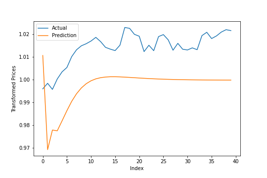

Image description.

It’s okay – it’s off by 1-2% for most of these estimations, which isn’t too bad. Of course, the important bit is how accurate it is when the data isn’t scaled.

unscaled_prediction = ref_scaler.inverse_transform(ref_prediction.reshape([-1,1]))
unscaled_test = ref_scaler.inverse_transform(ref_test_out.reshape([-1,1]))
mean_absolute_percentage_error(unscaled_prediction, unscaled_test)
## 4.092220035446507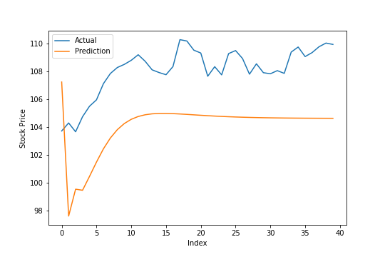

Once it’s unscaled, we end up with about a 4.1% MAPE. I’m not sure if that’s particularly good or not, but it brings us to the main question: How do the other stocks fare?

test_in_array = test_in.transpose()
test_in_array = test_in_array.reshape([*test_in_array.shape, 1])
test_out_array = test_out.transpose()
test_out_predictions = final_model.predict(test_in_array)
test_out_mape = mean_absolute_percentage_error(test_out_array, test_out_predictions[:,:,0], axis=1)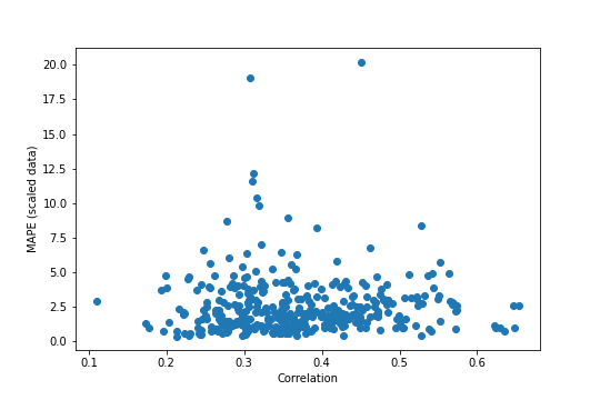

Image description.

It’s hard to tell exactly what is or isn’t there. It seems like there are fewer extreme MAPE values at both high and low correlations, but maybe that’s just because there are fewer points out there. We can try something a little stricter, by binning the data based on correlation and running an ANOVA on the bins (with a boxplot for visualization purposes).

import scipy.stats as stats  # for one-way ANOVA

levels = ["<0.2", "0.2-0.3", "0.3-0.4", "0.4-0.5", "0.5-0.6", ">0.6"]
cuts = [0,0.2,0.3,0.4,0.5,0.6,1]
correlations_boxed = pd.cut(correlations, bins=cuts, labels=levels)

corr_df = pd.DataFrame({"Correlation":correlations_boxed, "MAPE":test_out_mape})
groups = [pd.DataFrame(x)["MAPE"] for _, x in corr_df.groupby("Correlation", as_index=False)]
stats.f_oneway(*groups)
## F_onewayResult(statistic=0.859307579038562, pvalue=0.5086123809619022)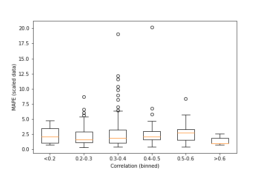

Image description.

A p-value of around 0.51 is much larger than any typical significance level, so it looks like there’s no statistically discernible differences between the above groups, despite the boxplot suggesting otherwise.

But this is all on the scaled data. What if it’s unscaled?

unscaled_out = lmms.inverse_transform(test_out_array.transpose())
unscaled_predictions = lmms.inverse_transform(test_out_predictions[:,:,0].transpose())
unscaled_mape = mean_absolute_percentage_error(unscaled_out, unscaled_predictions, axis=0)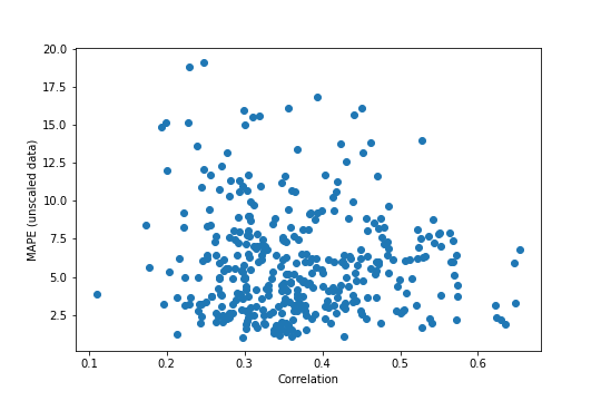

Image description.

The main takeaway from this – which could be seen on the reference stock – is that unscaling the data increases the MAPE by a lot, to somewhat worrying levels in a lot of cases. There’s still nothing very strong looking in this plot, especially with the MAPE values being considerably more spread out than before. It again looks like the higher correlations might not have as much spread, but it’s still tenuous.

unscaled_corr_df = pd.DataFrame({"Correlation":correlations_boxed, "MAPE":unscaled_mape})
unscaled_groups = [pd.DataFrame(x)["MAPE"] for _, x in unscaled_corr_df.groupby("Correlation", as_index=False)]
stats.f_oneway(*unscaled_groups)
## F_onewayResult(statistic=2.274528720161754, pvalue=0.046747350218964395)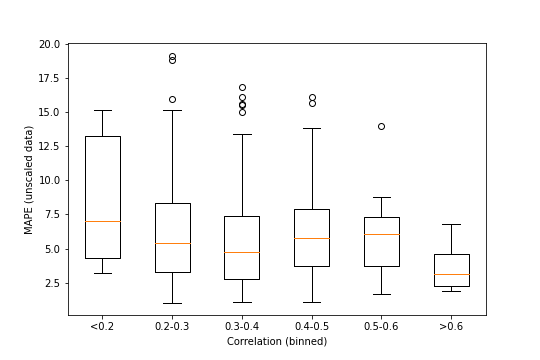

Image description.

The ANOVA is a lot more suggestive this time around, though. With p=0.047, this would be statistically significant for some common significance levels (including 0.05), though not all (it’s still above 0.01, for instance).

Conclusions

With this basic LSTM model, there might be some relationship between prediction error and stock correlation. Given how the MAPE values for the unscaled predictions on the non-reference stocks looked, there’s clearly work to be done on creating a more accurate model. Running this code a number of times would also be necessary to get a strong picture of the truth, given the random initialization that comes with neural networks.