Market Prediction with ETFs & Convolutional Networks

Convolutional networks are most prominently used for image analysis or on data with multiple spatial dimensions. Of course, since the inputs to the CNNs are all just numbers, you can feed in other data that has some a relationship encoded into the dimensions of the array. This post involves feeding data for historical returns from exchange traded funds (ETFs) into a CNN, and using it to try to predict the direction of the Dow Jones Industrial Average (DJIA) some time in the future. I’ll be using Keras to code the neural network. The Jupyter notebook used to develop this code is here.

As with all posts of this nature, this shouldn’t be taken as advice on what to do with your money.

Market Cycles and Sector ETFs

The stock market trends up and down over multi-year periods. Obviously, tracking the progress of these trends is of interest to economists and investors, so there are any number of ideas on how to monitor it.

Among those ideas is a sector-focused approach. Broadly speaking, companies can be sorted out into a handful of categories – sectors – like telecommunications or energy or consumer staples. The different sectors tend to behave in specific ways in different phases of the market, so looking at their recent collective behavior can provide insight to the market’s current phase and where it is more (or less) likely to go soon.

As Investopedia describes it:

Early in the business cycle during the expansion phase, for example, interest rates are low and growth is beginning to pick up. During this stage, investors or analysts who do a sector analysis would focus their research on companies that benefit from low interest rates and increased borrowing. These companies often perform well during periods of economic growth. These include companies in the financial and consumer discretionary sectors.

Late in an economic cycle, the economy contracts and growth slows. Investors and analysts will turn their attention to researching defensive sectors, such as utilities and telecommunication services. These sectors often outperform during economic downturns.

If you want to use sector analysis, then, you need some way of tracking the performance of the various sectors. Thankfully, there are ETFs which do that, with the SPDR (pronounced “spider”) ETFs being the more notable ones. There are currently eleven of these SPDR sector ETFs: Communication Services (ticker: XLC), Consumer Discretionary (XLY), Consumer Staples (XLP), Energy (XLE), Financials (XLF), Health Care (XLV), Industrials (XLI), Materials (XLB), Real Estate (XLRE), Technology (XLK), and Utilities (XLU).

They are not all the same age, however. Aside from the real estate and communication services ETFs, which appeared in October 2015 and June 2018 respectively, all the ETFs have data going back to December 1998. This is important in a bit.

The Problem

The goal is to be able to predict the direction of the DJIA some time in the future using the historical returns of the individual sectors over a window of time. Sectors all behave differently at different times in the market, so trying to use them all for prediction means being able to monitor their behaviors in parallel and spot large-scale patterns between some or all of them. These sorts of patterns are what convolutional networks are suited to detect, so it seems like one would be a good model more this problem.

The remaining part of the problem is what, exactly, to predict. Typically these kinds of problems end as either binary classification (i.e., will the DJIA be up or down?) or regression (trying to calculate what the value of the DJIA will be). I wanted to do something slightly different: a multiclass classification problem with three classes: “up”, “down”, and “inconclusive”. In this case, “inconclusive” refers to situations where the change in the DJIA’s value – up or down – over the period is within some threshold, maybe 2 to 3 percent, that’s considered small enough to be not worth bothering with. This is meant to create a buffer against situations where a binary classification model would predict that the DJIA would go up even though that possibility just barely wins out (e.g., 51% to go up, 49% to go down), while keeping it as a classification problem to keep the output easy to interpret.

Setup & Data Processing

First, import what we’ll need:

> import matplotlib.pyplot as plt
> import numpy as np
> import pandas as pd
> import pandas_datareader as pdr
> from sklearn.metrics import confusion_matrix, accuracy_score
> from sklearn.model_selection import train_test_split
> from tensorflow import keras
> from tensorflow.keras import layers
> from tensorflow.keras.models import Model
> from tensorflow.random import set_seed as tf_seed

> from api_key import TIINGO_API_KEY   # personal file with Tiingo API key

I got the historical data on the ETFs using Tiingo’s API. It doesn’t actually have the DJIA’s value over time, but it turns out there’s another SPDR ETF, ticker DIA, that is designed to track and correspond to the DJIA, so I used that in order to avoid mixing data sources. Plus, pandas_datareader has functions specifically for getting data from Tiingo’s API.

Additionally, as I said before, only nine of the sector ETFs had data going back to 1998. To ensure that there’s plenty of training data, those are the only ones I’m using. I don’t know whether or not the splitting off of the real estate and communication services sectors affects the predictive ability of the others, but I’m assuming that it’ll be okay and that there’s enough other data to not affect things too much. I’m also only taking data up to the end of 2019 to avoid the irregularities from COVID-19.

> FULL_ETFS = ["XLY", "XLP", "XLE", "XLF", "XLV", "XLI", "XLB", "XLK", "XLU"]
> full_etf_data = pdr.get_data_tiingo(sector_etfs, start="1998-12-22", end="2019-12-31", api_key=api_key)
> dia = pdr.get_data_tiingo("DIA", start="1998-12-22", end="2019-12-31", api_key=api_key)

Once the data is downloaded, it’s a matter of getting the returns from it. For the sector ETFs, each input needs to be a three-dimensional array of values with dimensions (length of the historical window) by (number of ETFs) by (one channel). We need one more dimension for the number of samples, so we ultimately need a four-dimensional tensor to store the input data:

> PAST_WINDOW_LENGTH = 250    # number of past days to use in prediction
> FUTURE_PREDICTION_TIME = 100  # number of days in the future to predict

> adj_closes = full_etf_data["adjClose"].unstack("symbol")
> adj_closes = adj_closes.values
> percent_changes = 100 * (adj_closes[1:,:]/adj_closes[:-1,:] - 1)

> data_length, n_etfs = percent_changes.shape
> n_entries = data_length - PAST_WINDOW_LENGTH - FUTURE_PREDICTION_TIME + 1

> daily_windows = np.zeros([n_entries, PAST_WINDOW_LENGTH, n_etfs, 1])
> for i in range(n_entries):
>     daily_windows[i,:,:,0] = percent_changes[i:(i+PAST_WINDOW_LENGTH),:]

The returns for the DJIA ETF are easy to calculate, but we need to use pandas.cut() to bin the returns into the appropriate classes:

> INCONCLUSIVE_LEVEL = 2.5  # in units of percentage points

> dia_close = dia["adjClose"].values
> dia_start = dia_close[(PAST_WINDOW_LENGTH - 1):(n_entries + PAST_WINDOW_LENGTH - 1)]
> dia_end = dia_close[(PAST_WINDOW_LENGTH + FUTURE_PREDICTION_TIME - 1):(n_entries + PAST_WINDOW_LENGTH + FUTURE_PREDICTION_TIME - 1)]
> dia_returns = 100*(dia_end/dia_start - 1)

> bins = [-np.Inf, -INCONCLUSIVE_LEVEL, INCONCLUSIVE_LEVEL, np.Inf]
> classes = ["Down", "Inconclusive", "Up"]
> dia_return_classes = pd.cut(dia_returns, bins=bins, labels=classes)
> one_hot_classes = pd.get_dummies(dia_return_classes).values

> dia_return_classes.value_counts()
Down             916
Inconclusive    1217
Up              2807
dtype: int64

As you can see, the classes aren’t balanced. But the market’s gone up more often than not between the end of 1998 and the end of 2019, so an excess of really good returns is to be expected. Since the smallest class still makes up about 18.5% of the data, I’m not going to worry too much about the class imbalance and just look at the confusion matrix as the primary diagnostic for the model. I am going to stratify the train-test split, though, since that’s easy enough that there’s no reason not to:

> X_train, X_test, y_train, y_test = train_test_split(daily_windows, one_hot_classes,
>                                                     stratify=dia_return_classes, random_state=1998)
> y_true = np.array(classes)[np.argmax(y_test, axis=1)]

Models

I tried three different network architectures for this problem – a basic non-convolutional network, a small CNN, and a larger CNN. Values I across all models are:

• Historical returns from the last 250 trading days (roughly one year on the calendar) were used for the input data.
• Predictions were made 100 trading days (around 5 months on the calendar) into the future.
• The thresholds for the “inconclusive” case were set at +/- 2.5% returns.
• All models were trained for 10 epochs.

Model 1: Basic (Non-Convolutional) Network

It’s best to start off with a simpler model, and despite what I said earlier, I don’t yet know if I actually need a convolutional network to do well on this problem. So it’s easy to throw together a model with a couple of dense layers and some dropout operations and see how well it works.

> tf_seed(1)
> model1 = keras.Sequential([
>     keras.Input(shape=[PAST_WINDOW_LENGTH, n_etfs, 1]),
>     layers.Flatten(),
>     layers.Dense(200, activation="relu"),
>     layers.Dropout(0.4),
>     layers.Dense(100, activation="relu"),
>     layers.Dropout(0.4),
>     layers.Dense(3, activation="softmax")
> ])
> model1.compile('adam', loss='categorical_crossentropy', metrics=['accuracy'])
> model1.fit(X_train, y_train, epochs=10)

> m1_predictions = model1.predict(X_test)
> m1_y_pred = np.array(classes)[np.argmax(m1_predictions, axis=1)]
> accuracy_score(y_true, m1_y_pred)
0.5036437246963563

…Not that well as it turns out. Despite having almost half a million parameters, it’s just a coin toss in terms of overall accuracy, and attempts to use a slightly bigger network didn’t really improve anything. Looking at the confusion matrix gives a clear indication that the model is excessively optimistic:

> m1_cm = confusion_matrix(y_true, m1_y_pred, labels=classes)
> pd.DataFrame(m1_cm, index=["True " + c for c in classes], columns=["Pred " + c for c in classes])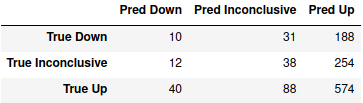

It correctly predicts that the market will go up the majority of times that it actually does, but it only gets about 5% correct when the market actually goes down. Overall, it predicts that the market will go up for 1016 of the 1235 test samples, or about 82% of the time. Considering how the DJIA was generally trending upwards for most of the data, this may be an understandable mistake, but it’s not doing us any good.

Model 2: Small Convolutional Network Over All ETFs

Next comes a very simple CNN: one convolutional layer that spans all of the ETFs, which then has its output flattened and the results fed to a softmax layer:

> tf_seed(2)
> model2 = keras.Sequential([
>     keras.Input(shape=[PAST_WINDOW_LENGTH, n_etfs, 1]),
>     layers.Conv2D(40, kernel_size=(30,9), activation="relu"),
>     layers.Flatten(),
>     layers.Dense(3, activation="softmax")
> ])
> model2.compile('adam', loss='categorical_crossentropy', metrics=['accuracy'])
> model2.fit(X_train, y_train, epochs=10)

The reason for having a convolution over all ETFs is because – to the best of my understanding – a pattern involving one adjacent pair of ETFs won’t be the same if it’s applied to a different pair, so applying filters to subsets of the ETFs would seem to be less effective.

> m2_predictions = model2.predict(X_test)
> m2_y_pred = np.array(classes)[np.argmax(m2_predictions, axis=1)]
> accuracy_score(y_true, m2_y_pred)
0.8153846153846154

> m2_cm = confusion_matrix(y_true, m2_y_pred, labels=classes)
> pd.DataFrame(m2_cm, index=["True " + c for c in classes], columns=["Pred " + c for c in classes])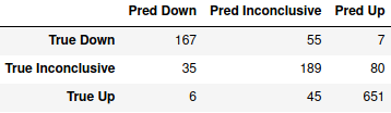

That’s much better, and with only about 37,000 parameters, it’s less than a tenth the size of the first one. Based on the confusion matrix, the model might still be a little too optimistic, though.

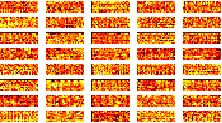
I made an attempt to try to visualize the weights in convolutional filters that the model came up with, but I’m not sure if it’s actually informative. There are clearly differences between the filters, but substantial patterns in them are hard to pick out:

I also tried looking at the activations, using code adapted from here. The data needs to be reshaped in this case since it comes out as a 221-by-1 array, and that’s difficult to visualize directly. But it can be reshaped into a 17-by-13 matrix and visualized with a heatmap easily enough.

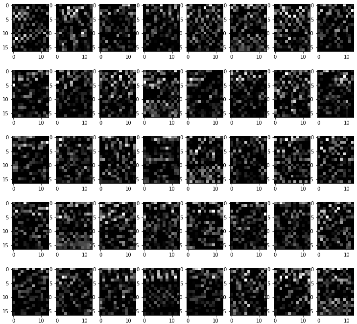
Even this doesn’t seem useful, though. Unlike with image data, the inputs for this don’t have a nice visual interpretation (especially since I had to reshape the data), so the picturing the activations won’t be much more comprehensible. There are several filters, like the top left one, which look like they’re maintaining fairly long streaks of every other point being noticeably activated, but I don’t have a sense of whether that’s real or it’s just seeing patterns where there’s not really anything to see.

Model 3: Bigger Convolutional Network

The third network I went for was a bigger convolutional network with more typical filter sizes. I wanted to use multiple convolutions here, and the easiest way to do that was to not do each convolution over all ETFs. Although I’m still using non-square kernels under the assumption that looking over longer stretches of time is still useful.

> tf_seed(3)
> model3 = keras.Sequential([
>     keras.Input(shape=[PAST_WINDOW_LENGTH, n_etfs, 1]),
>     layers.Conv2D(40, kernel_size=(5,3), padding="same", activation="relu"),
>     layers.MaxPool2D(pool_size=(2,1)),
>     layers.Conv2D(80, kernel_size=(5,2), padding="same", activation="relu"),
>     layers.MaxPool2D(pool_size=(2,1)),
>     layers.Conv2D(120, kernel_size=(5,2), padding="same", activation="relu"),
>     layers.MaxPool2D(pool_size=(2,1)),
>     layers.Flatten(),
>     layers.Dense(3, activation="softmax")
> ])
> model3.compile('adam', loss='categorical_crossentropy', metrics=['accuracy'])
> model3.fit(X_train, y_train, epochs=10)

> m3_predictions = model3.predict(X_test)
> m3_y_pred = np.array(classes)[np.argmax(m3_predictions, axis=1)]
> accuracy_score(y_true, m3_y_pred)
0.8955465587044534

> m3_cm = confusion_matrix(y_true, m3_y_pred, labels=classes)
> pd.DataFrame(m3_cm, index=["True " + c for c in classes], columns=["Pred " + c for c in classes])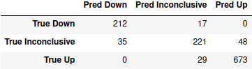

We’re back up to about 230,000 parameters here, which is still only about half the number in the first model. But it’s mildly better than the second model and still enormously more accurate than the convolution-less model. According to the confusion matrix, well over half the prediction errors are on the inconclusive cases, and almost all of the remainder are inconclusive predictions when things actually go up or down. I’m okay with this myself (at least, as far as I would trust this model with actual money), since I personally wouldn’t want to put any money down when the market is going more or less sideways, and fairly few of the up or down predictions have the market moving significantly in the opposite direction.

I can’t neatly visualize all of the activations for this model, since there are a lot of them and using padding="same" keeps the layers fairly large. I can get a few for one prediction in one image without streching anything, at least, so here are some activations from the first layer for one prediction:

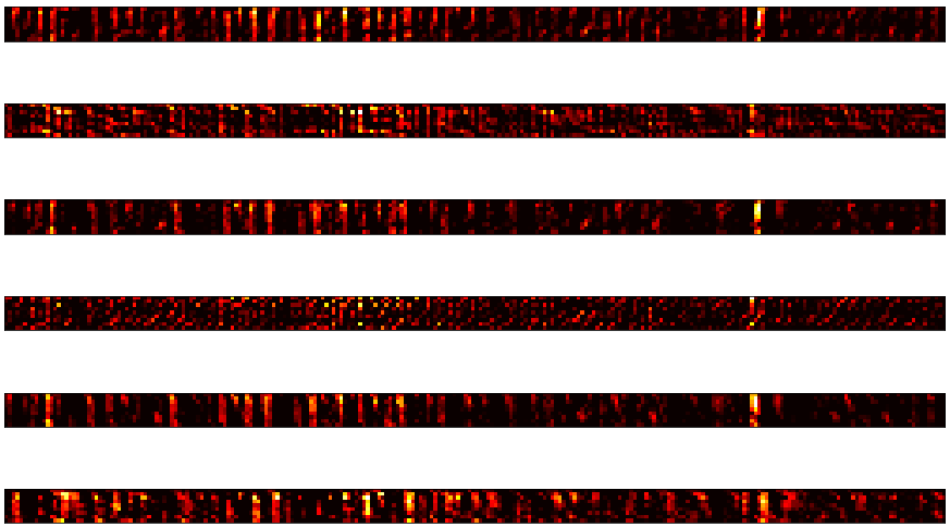
I said before that I thought that a convolutional window that went over all ETFs was needed, but the accuracy of this model and the patterns in the activations may suggest otherwise. (Although it’s a only modest increase in accuracy over the second model at the cost of six times as many parameters.) There are a lot of distinct bands in the first, third, fifth, and sixth activations. They also seem to have the strongest activations early on in the data (towards the left). I glanced at some of the other activations, and the other ones for this same prediction usually exhibit that same behavior; activations for other inputs didn’t necessarily do the same.

Conclusion

Convolutional networks, even fairly basic ones, do quite well on this problem. This is despite the fact that arrangement of the data along one axis of the input matrices is essentially arbitrary – I know of no particular reason why one ordering of the ETFs would be preferable to another.

I know that this model largely ignores the temporal component of each input matrix, and that there are models which are probably more suited to it. I’ve heard of LSTM-CNN hybrids that would probably do well, but I was struggling to find a good reference for it, so that’s something to revisit in the future.