An (Animated) Example of Bayesian Updating

Bayesian statistics is centered on constructing certain assumptions about how the probability of an event is distributed, and then adjusting that belief as new information comes in. It can be more involved to construct a Bayesian model as opposed to the “look at many things in aggregate” approach used in frequentist statistics. But it has nice properties, and we’ll take a look at them in a real albeit fairly unimportant context: the Pokemon video games.

A lot of video games have some sort of accuracy for their actions, and Pokemon is no exception. It is also commonly believed that when performing an action within such a game that has less than 100% accuracy, the accuracy check is rigged against them somehow. (Or that the game gives itself a boost in accuracy, but we’re not looking at that here.) But it’s often not that hard to just try it and see how often it works.

In other words, you have an initial belief to work off of, and then you can get data to update it. A pretty Bayesian setup.

Modeling

For this task, we’ll look specifically at the move Thunder. Various sources for the game claim that the accuracy of the attack is 70%, though for the purposes of this analysis, we don’t actually know that.

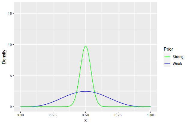
We start with making an assumption about what we think the accuracy is. Since the goal is trying to determine the probability of something, the |beta| distribution is probably the best choice for modeling it. For our initial guess of the accuracy, we’ll be a bit pessimistic and say that Thunder hits 50% of the time. For illustration’s sake, we’ll use two different priors: a weaker Beta(5,5) prior for the belief that the accuracy is probably around 50% but you’re not exactly sure and a much stronger Beta(75,75) prior for when there’s not much question in your mind.

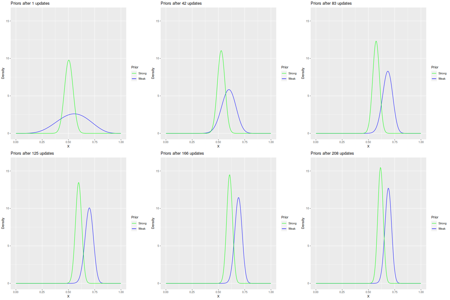
We then update the priors with the data we get. Conveniently, the updates are just Bernoulli trials, which is a |conjugate| of the beta distribution, meaning that starting with a Beta(\(\alpha,\beta\)) prior, if we update with \(m\) successes and \(n\) failures, the posterior will have a Beta(\(\alpha+m, \beta+n\)) distribution. This makes it pretty easy to calculate in R.

So after some testing, we come back with 208 trials with 145 successes and 63 failures. Updating the priors is fairly easy, and we can watch the update process thanks to the gganimate package:

The Final Posteriors

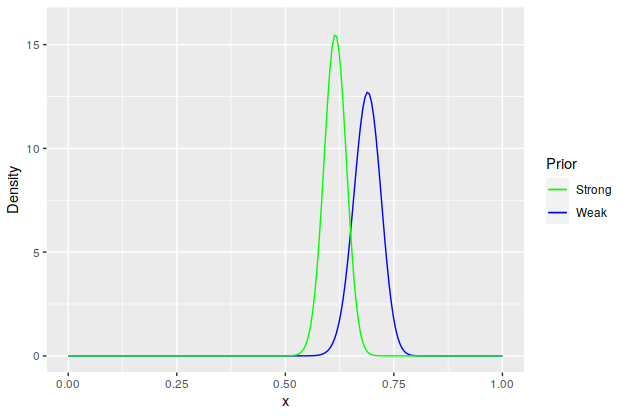
Of the 208 uses of Thunder, 145 of them hit, giving an accuracy of 69.7%, which is pretty close to the real value. A plot with some stats on the posteriors:

Prior	Posterior	Mean	99% Credible Interval
Weak	Beta(150, 68)	0.688	(0.605, 0.765)
Strong	Beta(220, 138)	0.615	(0.547, 0.679)

Note that while the weak prior’s 99% credible interval includes the sample accuracy, and in fact the mean is pretty close to it. The strong prior, on the other hand, is not quite there. It would doubtless be dragged closer to the 70% mark as more samples came in, but as it is now, it makes a decent anecdote about what happens if your very strong prior ends up being unrealistic.

The code used for this post is here.